Preprocessing Module

Overview

Preprocessing data means revising the measurement data to achieve an optimal reconstruction result. The SAFT algorithm is a mathematical operation that links result reconstructions linearly with the input data almost like a black box. There are some effects in the data that lead to artifacts in the reconstruction and that - if possible - should be removed from the data before the reconstruction.

Preprocessing is done at the user’s request. This means that all activities can be enabled and parameterized by the user.

“Select InterSAFT -> Tools -> Preprocessing” to open the small figure.

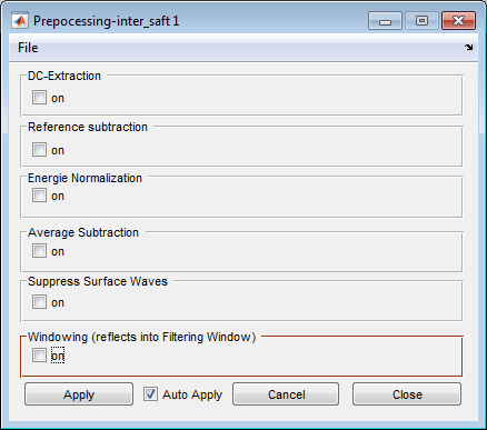
Preprocessing with all techniques disabled

Note:

Only in case of impulse echo data, the result of the preprocessing can be stored as ghk data files for further use.

DC extraction

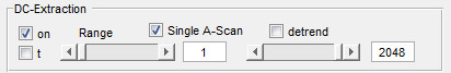
A DC value unequal to zero appears in many measurement data due to fluctuations within the amplifier preceding the analog-to-digital converter. The DC value calculated here is the average of the samples in the selected range and is subtracted from all A-scans from start to finish.

Parameters:
Single A-Scan	The average is treated for each A-scan separately
detrend	The average and small fluctuations are suppressed (use of Matlab function detrend). This operation takes more time and is usually not necessary if filtering is used.
Range 1	The range of the data to detect the DC value

Reference subtraction

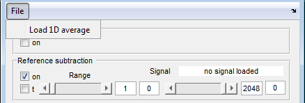
In many situation you will find that your transducer or your antenna has an ‘zero’ signal which is superimposed on all measured signals. This may come from reflections within the transducer or from the direct path of two antennas. The internal reflections within the transducer may be handled by deconvolution methods. Here you can subtract a reference signal which is loaded by “File -> Load 1D average” as ghk file, which you can produce by a small module from “Pundit Vision -> Select Module -> extract_reference”.

This feature allows you to subtract a reference signal which does not suppress backwall signals which are often common in all A-scans.

Parameters:
Range 1	The range of the reference signal which should be subtracted
Window Parameters	Tukey window parameters (0..1) which is applied on the reference signal before subtraction.

Note:

This feature subtract only one A-scan from all others. Therefore, it is not suitable for linear array applications.

Energy Normalization

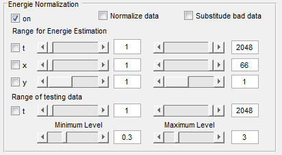
This sub menu allows you to select parameters for normalization and for substitution of bad A-scans.

1. Normalization: For ultrasonic data from measurement at concrete you will see very often that there are some or many A-scans which looks very different to others. This may happen if the contact to the surface is not constantly good or if there are irregularities near to the surface. This means that not all transmitted energy will reach the scatterers and therefore these signals are much lower in energy.

   With the module you may select a range in the data which should deliver comparable energy - this may be a backwall or only a late part of the data. The average energy in this range is then used to scale all A-scans to that value.

2. Substitute bad data: Sometimes it happens that single A-scans of a measurement are corrupted. For imaging perposes it is usualy better to have a similar A-scan than to have a bad or no A-scan. We try to find out - by energy consideration in a range of the data - which A-scan is corrupted and then, that A-scan is replaced by an average of the neighboring A-scans. The parameters specify the relative minimum and maximum value of the allowed energy of the tested A-scan to be identified as a “good” A-scan.

   Note:

   This method may not be useful for linear array data, since neighboring A-scans do not necessarily originate from neighboring measuring points. It is also obvious that an area of more than one damaged A-scan cannot be handled satisfactorily.

Average Subtraction

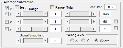
This technique may be used to simply suppress parallel structures in your data. To avoid that parallel structures in the geometry - like backwall echoes - are also suppressed, you may select a window by the definition of the range in t-, x-, and y-direction in which this average is calculated and subtracted.

Sometimes you only want to suppress low frequencies. Therefore an moving average filter can be applied to the average signal before subtraction.

Activating test means, that the range of the data is switched of by the window, so that you can see the influence in the main figure.

Surface Wave Suppression

The surface wave suppression function is very restrictive, but easy to handle. Surface waves are waves traveling between transmitter and receiver at the surface of the object under test. There are different wave types which may reach the receiver. Because of polarisation we have to distinguish between Rayleigh waves and SH (shear horizontal) waves. The SH waves are not realy surface waves, because the travel also into the volume, but the velocity in the region of the surface may be a little bit different because of material properties.

Rayleigh waves apear in case of SV (shear vertical) and P (preasure) wave excitation and they travel independent from volume waves with a velocity which is about 92% of the shear wave velocity. But the velocity of the Rayleigh wave depends also from the material in the near surface region and is therefore frequency dependent - that means: dispersive.

Because our signal is usually band limited and the distance between receiver and transmitter is near, we see always relative broad signals in the near time zone. Under the assumption, that the signal form does not depend from distance (this is not true because there are multiple point like transmitter and receivers combined in each device) we calculate an average of the delayed signals and subtract that signal from all A-scans. The width of the windowed signal is defined by the value w. The velocity of the wave is relative to the velocity used in the main figure (if vs == 1, we use the same velocity). A factor f ist used a multiplyer for the averaged signal. If we select f=0, then the signal is not subtracted but the signal is multiplyed by an inverse window function, which presses the values to zero at the expected time delay.

Parameters:
test	Use a small window at the expected time, to detect the correct velocity
act	Activate the suppression
vs	v_surface = vs * main_velocity
f	multiplication factor before subtracting the averaged signal. If f==0: cut the data to zero within the window
w	Width of the window (precalculated by the signal center frequency w = 2*/f_0 )
norm	The signal is normalized to the actual A-scan energy in the window, before the subtraction takes place
4 Number fields	Definition of borders on the surface by two points P1(x1,y1) and P2(x2,y2)

Note 1:

It is assumed that the signal is damped by \({ 1} \div {\sqrt{ distance }}\). If there is an overdriving of early arrivals, this may not be true. The factor has to be adapted accordingly, or has to be set to zero.

Note 2:

There is an additional surface wave module (SurfaceWaves) with which the surface waves can be analyzed much more precisely. This module can be called from InterSAFT and sets the selected B-scan for analysis. (The suppression of surface waves in SurfaceWaves is not immediately reflected in InterSAFT. A new modified measurement dataset must be created during the operation.)

Windowing the signal

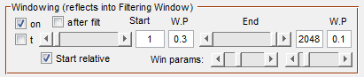
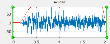
Result of windowing displayed in filtering figures. Example: Left and right slope are different (0.3, 0.1). The start is delayed according to the distance from transmitter to receiver.

This tools allows to switch the data smoothly on and off for a fixed time range or for a dynamic start point. The values of the range are given as index to samples. The number of samples are the number of samples selected during reading the file (usually the full A-scan length) multiplied by the oversampling factor ov_t in the main figure.

Parameters:
Slider 1, Start	Starting sample of the left window border
Slider 2, End 1	Ending sample of the right window border
W.P.	Windows parameters (Tukey window) for left and right window slope
Start relative	If set: the left window border depends on the distance between transmitter and receiver for each A-scan separately.
after filt.	If set: the windowing process is done after the filtering process.

Note:

Window parameter = 1 means, that 50% of the range is used for the up going / down going slope.

1(1,2,3)

With rev. v729, the definition of end of range has been changed. If “End” is the last sample, this value means the end of the A-scan for all other A-scan lengths, which may be used with this setting. This is important if you want to use the actual setting as a default setting.