Getting started with InterSAFT

Useful information in advance

The name InterSAFT stands for an interactive SAFT reconstruction tool implemented in Matlab. It should be user-friendly and contains a multitude of built-in functions for the reconstruction of defects in isotropic and anisotropic media.

The SAFT and FT-SAFT algorithms and some variations are used as imaging methods. For the result of an imaging procedure in ultrasound technology the term ‘reconstruction’, which we usually also use here, has become established.

In addition, we speak of A-scan (or A-scan) for the result of a single ultrasound reception. Many A-scans are combined into one measurement file and are then often called B-scan. But here, a B-scan (also B-scan) can also be the result of a reconstruction, whereby the time was already converted into a spatial variable (usually the z-coordinate).

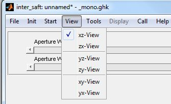
In case of a volume reconstruction R(x,y,z) we speak of xz-B-images or yz-B-images, whereas the xy image is called C image (cross section parallel to the measuring surface that lies in the xy plane).

The measurement coordinate system (local coordinates) is understood in such a way that the x-coordinate denotes the scan direction and the y-coordinate the parallel scan lines. The z-coordinate is directed negatively into the body. The counting direction is thus a standard right system on the measuring surface, with the 1st point at the origin of the coordinate system. The actual position of the measuring points can be adapted to this system by offsets and negative step widths in the ghk header.

How do you perform a calculation?

Working with projects

Working with projects should facilitate the concentration on a certain task, a certain type of measurement, with a defined device. When you start InterSAFT, an unnamed project is created, which can be saved at any time and contains all parameters of the calculation and display of the actual state. Data and results are not saved in a project file, since the recalculation usually takes only seconds. When saving an executed reconstruction, the state of the current project is automatically saved in a file <name_of_the_reconstruction>.spb.

Loading a project at a later time requires the data again and should lead to the same results as before after a recalculation. The project file is saved in the standard Matlab format and can be read into Matlab, modified and saved again using the corresponding load or save calls. (To ensure that Matlab does not interpret the extension of the file name incorrectly, the ‘-mat’ option must also be specified).

Preparatory work:

• Make sure that your data is in a ghk file format (or raw/lbv/sdd), otherwise the data must be converted to the ghk format. Tools exist for this purpose: (rf_header can be called by e.g. Pundit Vision -> ‘edit header’). The ghk file format contains all basic information for reading the binary data and for positioning in a local or global coordinate system. The input data for a reconstruction are A-scans, therefore only such data can be used here. The data must be available in the time domain.

• For the use with linear array measurements a further file with the extension .sdd is required, which describes the connection of measurements at different measuring positions.

• In order to provide a quick access to known binary data, such files (ending .raw or .lbv) are also accepted in connection with a ghk header file. Different default settings are stored in so called ‘default headers’ in the user_settings directory. When using preset projects, corresponding header files are offered automatically when loading raw or lbv files.

Right from the beginning:

• Start the InterSAFT module from Pundit Vision.

• You will be prompted to select a project template. There are templates for different measuring instruments which are supplied with a certain program version or which were created by the user himself. In addition, you can select a previous project directly via the file selection. (While the select_preset panel is displayed, the display of Pundit Vision temporarily disappears.)

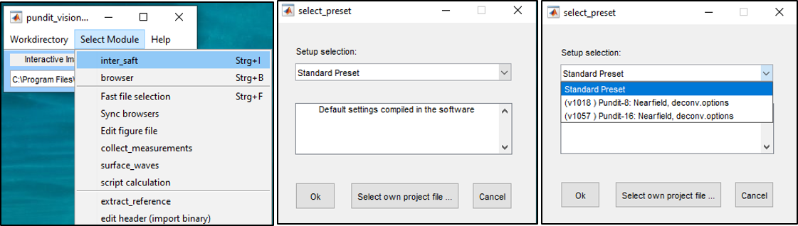
• If you call one of the listed project templates (presets), you can then load an A-Scan file via ‘File -> Load Data (ghk)’ or ‘File -> Load Data (lbv/raw)’. You have the possibility to restrict the data range (range_definition), but this is usually not necessary. If you select a previous project, you will be asked if you want to load the data from the previous project. If you deny this, only the parameters of the project settings are applied and you can reload other data and process it with the settings of the previous project.

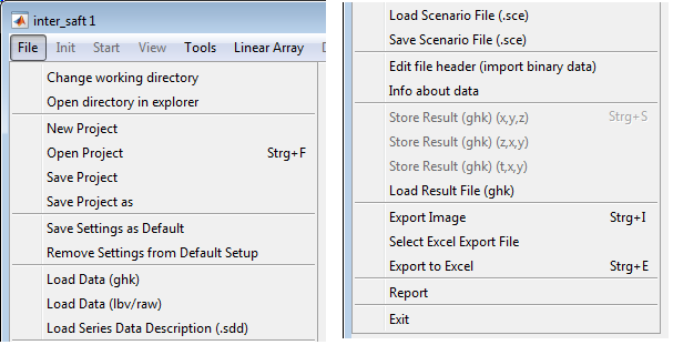
Input and output operations in the file menu

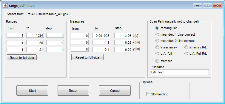
Range-definition window: Selection of a data area within the measurement file.

Note:

When the Range-definition window opens, the values of a previous session are displayed. You can reset to the full size of the measurement area (Reset to full size -Downsampling is retained) or to the full data (Reset to full data - also Downsampling is reset). After making changes, you can use “Reset” to return to the original values. The information under ‘Scan Path’ is for informative purposes only. The settings result from the file header and should not be changed. Changes are only temporary and can lead to error situations.

• After reading the data, the data parameters are known to the software. After loading data for the first time, the reconstruction parameters must be adjusted with “Init”, this also happens without prompting if you use ‘Start’ directly. If you want to exchange the measurement data by new loading and keep the settings of previous reconstructions, “Init” is not intended, but also no longer necessary.

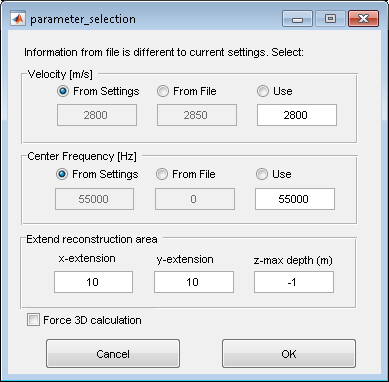
Init window: Initialization of the reconstruction space settings. The setting ‘Force 3D Reconstruction’ is only possible if the corresponding option is available.

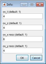
It is possible that another window opens (Info:) indicating that parameters of the current project setting do not match those of the default project setting. This is only a hint to draw attention to possible misadjustments. (The project default settings can be set under Tools->Options->Basics and saved under File->save settings as default.)

• Now you should check some parameters:

  • The speed of the background material.

  • The size of the reconstruction area.

Note:

The distance of the pixels in the SAFT or FT-SAFT reconstruction is identical to the distance of the A-scans in the scan aperture. If you increase the number of points in the reconstruction, the size of the reconstruction is automatically adjusted. This applies only to x and y coordinates. The distance of the pixels in the z direction has no limitation. You can choose the size and number of points accordingly. If you want to increase the number of pixels manually to a much bigger value, this may have to be done in several steps. The reason for this is that the interactive mode of operation should not come to a standstill due to incorrect input, i.e. without the real wish of the user.

• • By entering an oversampling (interpolation / oversampling > 1) in the panel of the reconstruction space specifications, the reconstruction space is resolved by the specified factor higher than the distance between the measurement points. However, this also means that the file size of the result and the computing time increase accordingly. In linear array applications, the spatial sampling rate refers to the distance between the individual sensor elements in the array.

    The values under ov_t, ov_x and ov_y in the aperture panel refer to an interpolation by increasing the spectral range (fft interpolation). The interpolation of the time domain improves the result of the reconstruction to a certain extent if the spatial resolution is high. The interpolation in x- and y-direction improves the reconstruction result essentially in the near range. Since with linear array data local interpolation cannot be performed so easily and unambiguously, the parameters have a different meaning:

Note:

If the interpolation in the local area (ov_x / ov_y) is selected to be as large as the oversampling specification of the reconstruction space, the interpolation can usually also be performed on the result. This saves computing time and memory space and can be performed in the browser module during visualization. (The effects of interpolation can be observed in the spatial range and in the spectral range (selection: spectrum dim1 +2). Falls die Interpolation im Ortsbereich (ov_x / ov_y) genauso groß gewählt wird wie die Oversampling-Angabe des Rekonstruktionsraums, kann die Interpolation i.R. auch auf dem Ergebnis erfolgen. Dies spart Rechenzeit und Speicherplatz und ist im Browser bei der Visualisierung durchführbar. (Die Effekte der Interpolation lassen sich im Ortsbereich und im Spektralbereich (Selektion: spectrum dim1 +2) beobachten. Note that the resolution is always associated with the spatial bandwidth given by the center frequency and speed or with the wavelength.

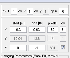
Definition of the reconstruction area: For 2D reconstruction: Depending on the selected view, only those values are accessible that define the visible view. All values are activated for 3D reconstructions.

Here we go:

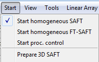
• Now you are ready to start the calculation: Select Start -> Start homogeneous SAFT or Start -> Start homogeneous FT-SAFT for 2D reconstruction or ``Start -> Prepare 3D (FT)-SAFT for 3D calculations. Only 2D calculations are performed interactively.

Start of the calculation after loading the data.

• 2D SAFT and 2D-FT-SAFT: The selection of Start homogeneous SAFT starts the interactive calculation mode. This means: Every change of the parameters now visible on the screen leads to a new calculation and display of the reconstruction result. (The function for calculation with the FT-SAFT algorithm is not available in every distribution).

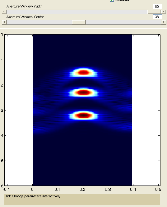
Example of a 2D-SAFT reconstruction of a concrete specimen

• You can choose which slice you want to see or which view of the volume is displayed. The display of the data can be influenced by numerous display parameters.

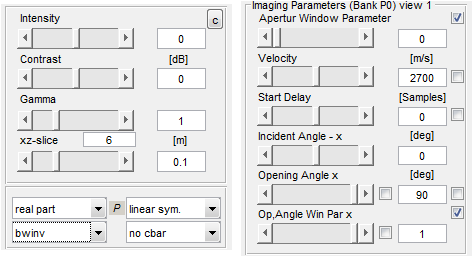
Left: Options for changing the display; Right: Reconstruction parameters.

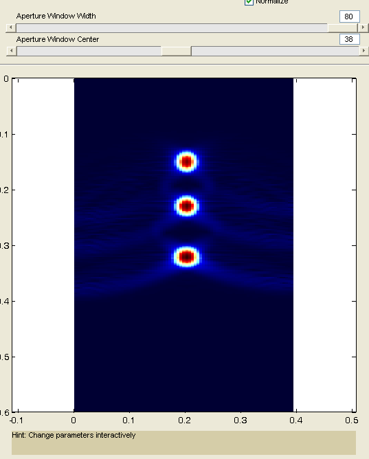
Aperture Window

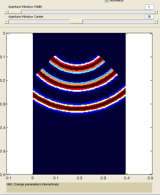
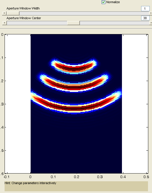
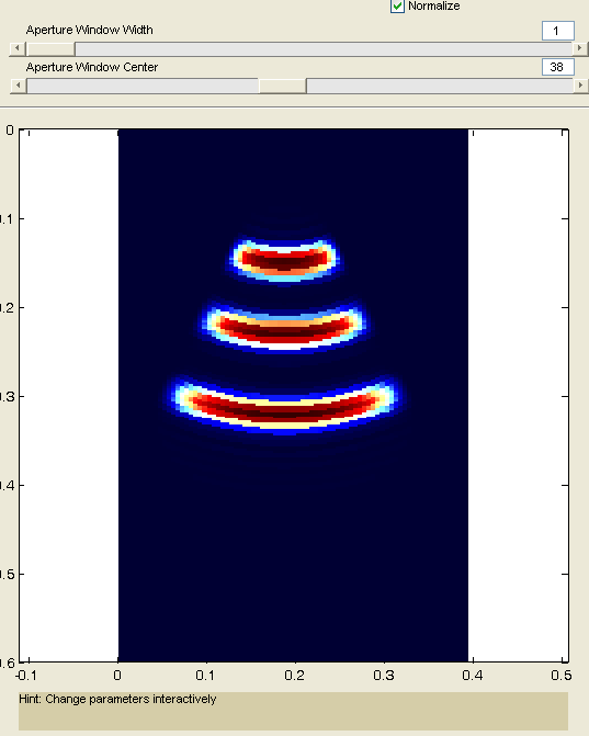
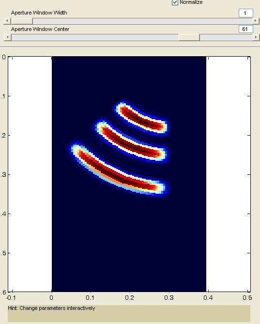
• The most important feature of InterSAFT is the observation of the effect of imaging algorithms on the reconstruction of scatter indications depending on the quality of the data and the parameters of the imaging algorithm. You should observe how the image changes when the aperture parameters are changed.

Opening Anlge 45° Op.Angle Win Par x = 0	Opening Anlge 45° Op.Angle Win Par x = 1	Opening Angle = 20°
Opening Angle = 20° Incident Angle = -20°	Opening Angle = 25 °, alle A-Scans	Opening Angle = 50 °, alle A-Scans

Reconstruction with 3D-SAFT or 3D-FT-SAFT

If 3D-(FT-)SAFT is selected, the interactive calculation is deactivated. Now you can change all menu parameters before selecting Start 3D SAFT. In FT-SAFT mode, this forces all data to be read again. (You can re-select a portion of the data) and 3D processing will be performed. When the calculation is complete, a new mode appears in the main window: the Display-only mode of the main window.

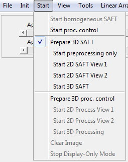
Activating the 3D (FT-)SAFT mode offers the possibility to change parameters and start 3D processing.

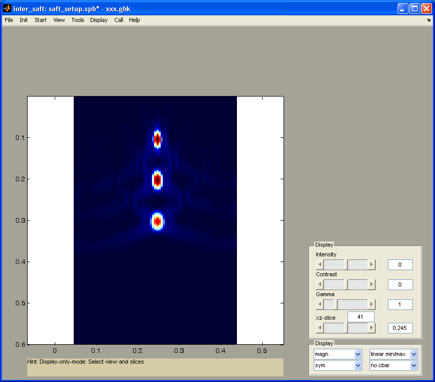
Display only mode of the main window. The background color is changed. The interactive recalculation is switched off.

If this mode is selected, only the visualization of the result is possible. Changing the reconstruction parameters is disabled. However, you can switch the visible section through the 3D data by selecting the view.

In the pure display mode only some limited actions like changing the view (selecting the cutting direction) View are possible. No recalculation is performed.

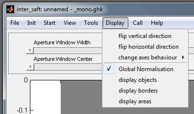
Display options in (Display only mode).

The reconstructed data are stored in the main memory of the computer and can now be stored in a file on the hard disk for later use. (File -> store result (ghk)). Another possibility of visualization is to call the module “Browser” on the data (Call -> call browser on reconstruction). To do this, the reconstruction data must be saved on the hard disk. If this has not yet happened, you will be prompted to do so.

Note:

Remember to save the reconstruction. After leaving the ‘Display only mode’ this is no longer possible.

Call the 3D visualization module “Browser” to display the data or the reconstructed volume.

The pure display mode is ended by pressing Start -> Stop display only mode. The data and the results are no longer valid in the memory and must be reloaded or calculated. There are exceptions to this: If the reconstruction was carried out in steps the 2nd stage can be started after the 1st stage if the result of the 1st stage is kept in the memory. This will be indicated interactively.

Exit the pure display mode in the Start menu “Start”.