program handling with reconstructions of linear array data
After starting the program, the empty main menu appears, which can be resized at any time by dragging the edges.
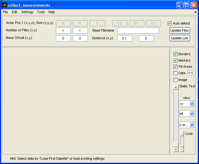
main window
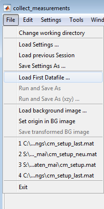
Step 1: Open a base file from which the name for the file series can be determined: File -> Load First Data File. If this is a series of files, a file that contains a 1 in the name must be selected.
registry for the data selection
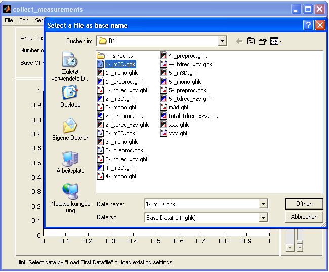
data selection
In the example, it is the file 1-m3d.ghk, which was created as a result of a 3D reconstruction of InterSAFT. The time range data can be edited in the same way as reconstruction files. After opening this file, the detected file series will be displayed in a list. Here it is possible to remove files from the list or select them individually. If not all files are displayed in the list, this may be due to the fact that files are missing in the numbering, which then led to the abort of the list determination. This problem can be solved later by editing the names of the respective file.
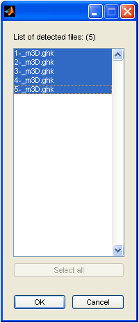
data list
When all names are correct, there is nothing to change in the list. After the submission, the base data and the derived amount of files appear in the main menu. The name of the base file includes the #-sign in place of the progressive number. The usage of decimal numbers with multiple digits is allowed. Up to 3 decimal digits can be recognized, where the number may be put behind zeros e.g. (x_001, …, x_009, x_010 etc. or x1, …, x9, x10 etc.)
Step 2: Definition of the starting coordinate and the distance between the single measurement files.
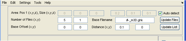
placement of the data series
With the automatic file name generation, the #-sign for the file number’s place holder can be changed manually. After that, the file list is restarted by specifying number of files. There, the amount of the entered numbers must contain at least the last file number. Files which are not found in between or at the beginning are then excluded from the displayed file number. Files, which are not automatically detected, must bee added in the file table manually (right mouse button in the file table).
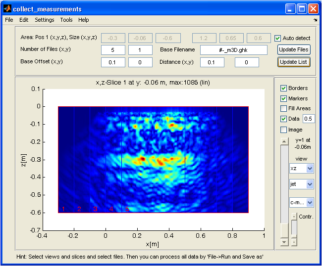
By clicking Update Files the files are read, analyzed and an overview in the geometrical arrangement is displayed in the main window. The selection is done by the options Fill Areas and Data. In the following example the files are strongly overlapping, because the x-offset between the files is 0.1 m and the reconstruction space is 0.8 m wide.
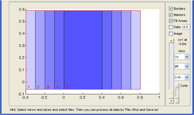
data fields in the coordinate system
By default, Fill Areas may be selected, that means that the area of every single file are initially colored and semi transparent displayed. The overlap may give the impression that different areas overlap especially strong. This impression is not really important, since the true data under the linear array only extends 0.2 m in the x-direction and this data overlaps only once at an offset of 0.1 m. (The information varies of course with different experiments and devices.)
Step 3: Depiction of the overlapped data
In the main menu following options can be selected:
Borders: The borders of the data areas
Markers: A numbering and marking of the data areas. By clicking the markers (left mouse button) the corresponding data can be switched on and off directly (similar to Activate in the file table). By clicking on the markers with the right mouse button, the corresponding file is switched to solo which means that it is shown alone or it is shown with other solo switched markers. By clicking the marker switch multiple times, the color of the nonactive data markers can be changed.
Fill Areas: Depiction of the data areas as filled transparent area
Data: Depiction of the data switched on/off. The number value next to the button is the transparency value of the data when it should displayed together with a background image.
Image: Activation of a previous selected background picture
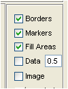
visual options
The slider enables the view on different 2D layers and to work on them. Depiction options:
view: xy, xz, yz
Farbtabellen: jet, bw, …
Datentyp: real part, imaginary part, amount, …
Kontrast: Setting of the contrast by a multiplicative factor
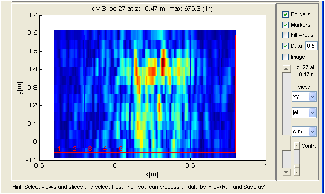
data fields with active data display
It is important to ensure that the images overlap correctly. By changing the sign of Offset and Distance (see following picture), this can be adapted without changing the original data.
data overlapping to the right progressively
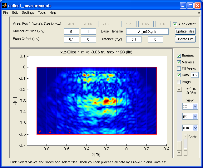
data overlapping to the left progressively
After changing the offset values, Update List must be clicked to submit the changes on the positions of all files.
Step 4: Operation of the calculation and saving the result
To create a data set which contains all the data layers, the menu point File -> Save As has to be called. After specifying or selecting a file name, the calculation is performed. Because of storage reasons, the data in z-direction are processed as layers and are stored progressively as (x, y, z) data fields. This is why an interpolation of the data is only provided for the xy-view. By default, a linear interpolation is performed. This can be changed under Settings->*Interpolation*.
Specifics: If the data are not arranged regularly, every single offset can be corrected manually. To do this, a separate table must be called in Edit -> File Matrix. The example then shows:
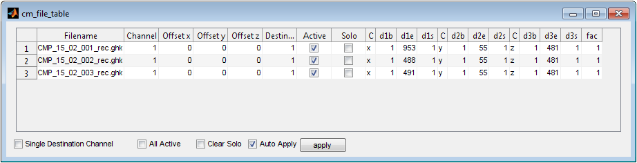
file table
Where the offsets x, y, z can now be manually changed for each file. The default setting results from the offset of the main menu. In the table following entries can be changed:
Meaning of the entries in the file table:
Channel: The data in a ghk-file can have more than one channel. Channels are data fields in the file, which can come form different probes, for example. Because of the channel structure every file‘s data field have the same structure, size and coordinates. Normally the number of channels in one file is 1, so the channel parameter of the data is set to 1.
Offset x, Offset y, Offset z: Additional shifts of the coordinate system of a file. The Coordinates of the ghk files stay effective but are corrected by offsets.
Destination: You can display multiple reconstructions in different target data fields by adding multiple ghk files to the data table and setting a different value under Destination for each file. The default value for Destination is 1. All data fields have the same transparency, the same contrast and show the data of the same 2D slice. The data fields are also numbered in the left bottom corner. In the following figure 3 destination data fields are shown, which are shifted side by side by an extra offset.
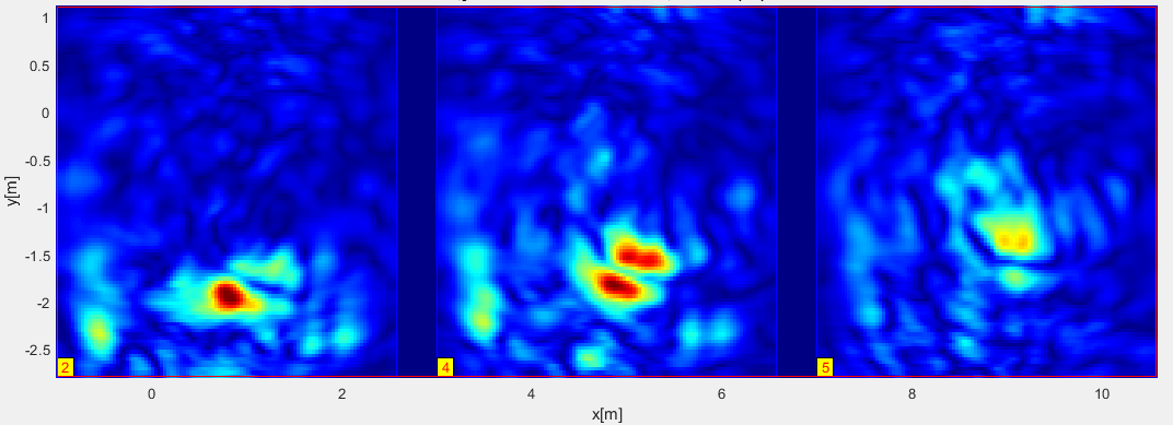
destination fields side by side (by Offset x=4m)
The use of destination channel is very flexible. The possibilities are selectable in the main window under Settings -> Channel Coloring. There are colour codes but also vector representations to choose from. The default setting is: Channel 1 -> red, Channel 2 -> green and Channel 3 -> blue. The result shows a colored visualization with mixed colors at the locations, where the information varies. Color-coded angles and vector arrows are provided for the representation of polarizations of a vector field.
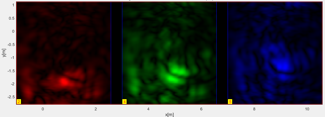
destination fields separated in RGB
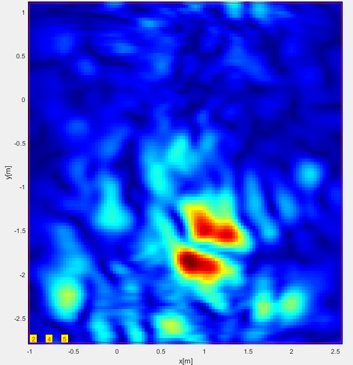
destination fields in single channel
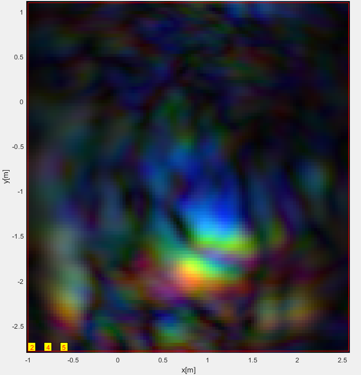
destination fields overlapping in RGB
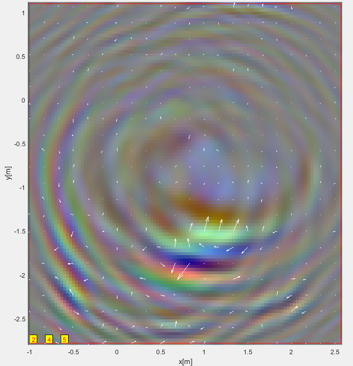
destination fields used as vector components
With single handling data (in the global coordinate system) that overlap in the image, the colors are not mixed. Their colors are covered over another by their transparency, instead. This is comparable with a stack of colored, self illuminating window glasses. For a more advanced editing of superposition and mixes of channels, the actual visualization can be exported in separated files into the working directory and being overlapped by an editing software e.g. Inkscape or Photoshop (Tools -> Export Image Components). In Inkskape, the colored data fields must be put in different layers over another and set them to Screen Mode. The colors will be mixed additively and a white color mix results.
Single Destination Channel: This button is used to temporarily combine all destination channels into a single channel where the data is displayed in the specified color table. The assignments to the channels in the table stay registered and will be reused after deselecting the option.
Active: Activation of the usage of the respective file. (Alternative: marking in the main window).
Solo: Temporarily switches off every data except the one (ones), which is (are) marked with Solo. This allows a quick orientation about the effects when superimposing the individual files.
Auto Apply: If this switch is set, the changes in the table (except for changes to the file name) are carried out immediately.
Adding and deleting data files: Clicking the right mouse button in the table opens a context menu. There you can reach the options Add file or Remove selected file. After clicking apply, the changes in the table are then displayed in the main menu.
C (name of the coordinate), d1b (Starting Index), d1e (Ending Index), ds1 (Stepwidth), analogous entries for the coordinate 2 and 3: Display of the area from the data file, which is brought to the visualization. The area selection originally takes place at the first opening of a file, but can be changed afterwards.
Fac: Factor with which the respective file is included in the total.
Step 5: Including a background image
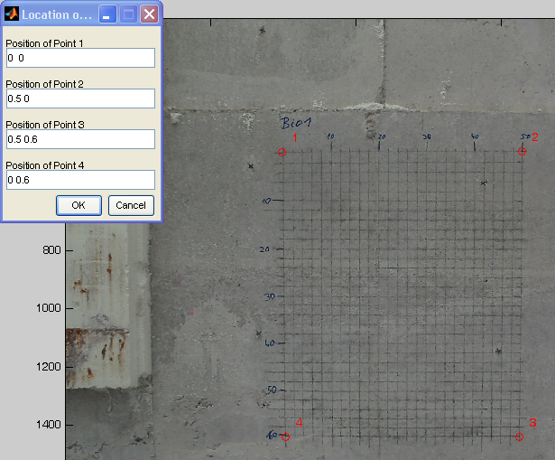
For better orientation and documentation purposes, the presentation of the data can be mixed with images or plans of the measuring arrangement. This means that the data can be inserted into a photograph or a plan with local accuracy. For this purpose, a photograph must be perspective corrected and adapted to the coordinate system. The user has to mark four points on the image and define their coordinates in the measurement coordinate system. This is realized quite simply in the program: Open the menu item File -> Load Background Image. (The image file does not have to be in the current working directory. The working directory is also not changed by the file selection). The image will then appear in a new window (which can be resized). In the image you can mark exactly 4 points by clicking on them. (In case of wrong entries the procedure must be repeated.)
After entering 4 points, a small table appears in which the coordinates (e.g.: 0.5 0.6 for x=0.5 m and y=0.6 m) are entered. The marked coordinate points are circled and numbered red in the image. After entering the coordinates, the image is rescaled, rotated and aligned, which can take a few seconds. Then you can limit the image section to be used by entering coordinates in the measurement coordinate system. A table appears with the presettings of the corner points, which result from the extent of the photography. Thus, if one wants to use the complete image, one simply continues with OK.
entry of the the background image’s coordinates
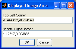
positioning of the background image
The image window is then closed again and the background image can be switched on in the main window by activating Image. The data is placed in front of the image at the corresponding coordinate by specifying a transparency (0..1). However, the image is only displayed in the xy view of the data. By clicking on Settings -> Axis equal or -> Axis tight you can adjust the axes of the coordinate system of the display. Since this work on an image file is a bit time-consuming, the result image can be saved as a jpg file (File -> Save transformed BG image). The jpg image contains the already rectified image and the coordinates of the total extension in comment fields. If you load this image again later, the comment will be evaluated and the image will be displayed in its original coordinates (File -> Load background image). The origin of the image coordinates can be adjusted later to the origin of the data fields in the files (File -> Set origin in BG image).
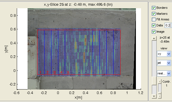
destination data fields with background image
Step 6: saving the settings
By File -> Save Settings the current settings are saved in a project file for later reuse. The background image and its scaling are contained in the project file, while the data files are only saved as a reference in the file table. Therefore, the data and the project file always have to be in the same directory, whereas the original image is not longer needed.
Particuliarity: Incorrect file numbering If there are problems with reading the files from the base file, as mentioned above, it may be because files are missing in the serial numbering. The automatic detection then fails. The only reason for this is a lack of information, which can easily be supplied to the algorithm. In the main menu, set the number of files in x-direction (Number of Files (x, y)) to the last number of the progressing data series (not to the amount of files!) and the data list will be determined automatically and the missing files will be skipped. The automatic generation of the starting positions of the files ignores the number in the file name and advances the starting position continuously. This can be tracked in the file table and corrected manually if necessary.