Surface Waves

This is a short introduction to the use of the inter_saft utility “surface_waves”

Start

The “surface_waves” module can be started from Pundit Vision or from InterSAFT in a synchronized mode.

Import data

Data must be available in “ghk” Ascan format (dimensions: time, space, space). Open the file: “File” -> “Load Data File”. Then the known panel for selecting a subset of the file appears.

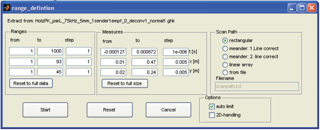
selection panel

The entries are self-explanatory. With “Start” the inputs are accepted and the selected sub-matrix or the complete file is loaded and displayed directly.

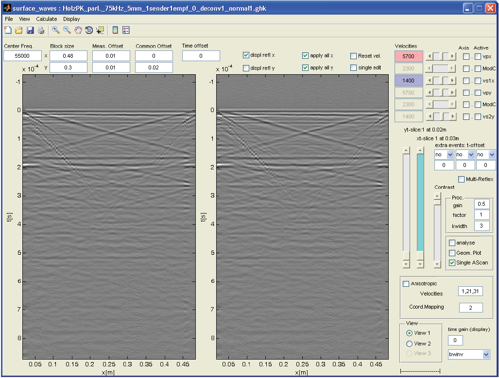
display of loaded file

Display parameters

Section of the view (“View 1” or “View 2)

The ghk file contains A-scans which are displayed parallel to the 1st scan axis (View 1) or parallel to the 2nd scan axis (View 2) according to B-images. It should be noted that currently the scan axis 1 is always called x-axis and the scan axis 2 is always called y-axis - regardless of the name in the file, which normally appears in the name of the axis in the menus.

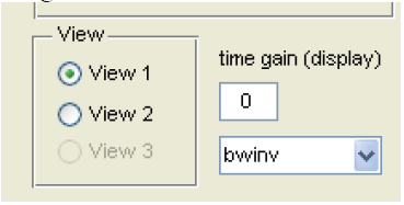
view selection

Beside the view selection you can select the color table (jet, bw = black/white, bwinv = white -> black). In addition a parameter is provided as TimeGainCorrection, which multiplies the A-Scans depth-dependency with “t^gain”. So: gain=0: not amplified, gain = 1 : linearly increased etc.

1.3.2 Selection of B-scan and contrast

The two sliders “yt-slice” and “xt-slice” can be used to select the slices of the respective view. The currently active slider is highlighted. The other slider is required for manual speed adjustment. Next to the sliders for the slices there is a “Contrast” slider that changes the level of the color table. This means: if the slider is set to 10 %, the maximum of the color scale is already reached at 10 % of the amplitude in the data. Thus the contrast is always higher with small slider values.

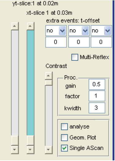
B-scan and contrast sliders

Set parameters

Geometry and correction of specifications in the data

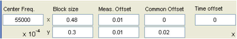
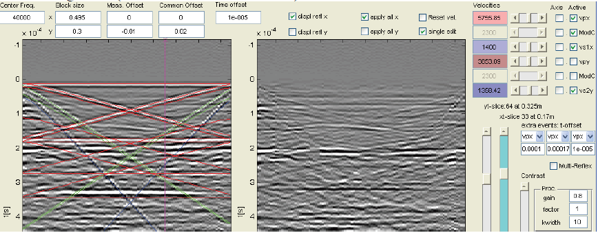
data settings

Above the B-screens are the entries for the:

1. Center frequency of the signal: From this information, the width of an analysis band for the display suppression is determined.

2. Block size: Expansion of the surface of the test block to be examined.

3. Meas.offset: Correction values for the position of the coordinate system on the test block. These values are added to the values in the ghk file.

4. Common Offset: Distance between the Transmit Probe and the Receive Probe for Pulse-Echo Measurement

5. Time Offset: Correction of the start time of the data regarding the specifications in the ghk file.

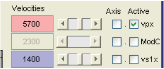
Velocity selection

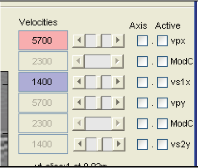
speed selection

The surface waves that appear in the measurement data are partly actual “surface waves” and partly space waves that “hit” the surface or form the visible part of the space waves on the surface.

Based on current experience, 3 wave speeds are planned.

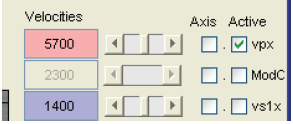
The fast p-wave here is referred to as vpx here because the portion that runs in the x-direction is the vpx.

A mode-converted wave formed by the p-wave to the edge and the s-wave running back.

A slower surface wave - here the Rayleigh wave, which runs in x-direction and is reflected at the y-edge (vs1x), if the excitation polarization takes place in x-direction. Or an s-wave, if the excitation takes place in y-direction.

vpy : p-wave running in y-direction.

Mode-converted wave in y-direction

vs2y: s wave running in y direction. Depending on the excitation polarization, this is a true s-wave or a Rayleigh wave.

The speeds of the waves can be adjusted by a slider or by a numeric value. The “Active” button can be used to activate or deactivate a wave type. With the button “Axis” you can convert the t-coordinate in the right B-image to a spatial axis (z-axis) and display it, so that you can directly read a depth indication for displays in the data field.

For further selection of speeds: see below.

Perform calculation

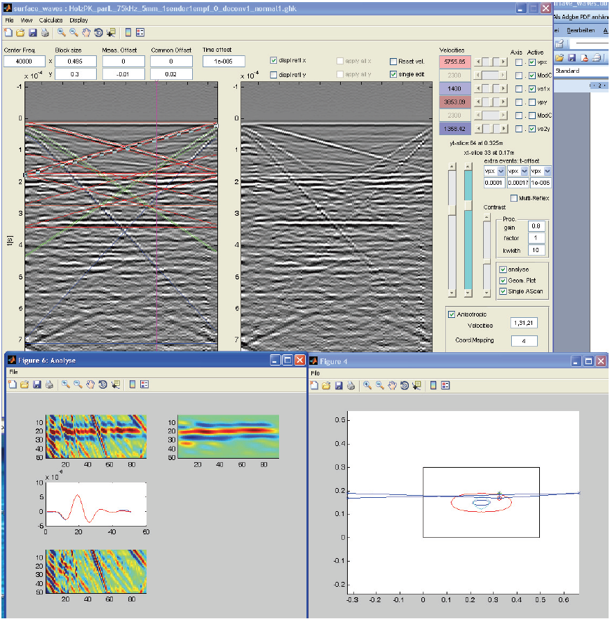
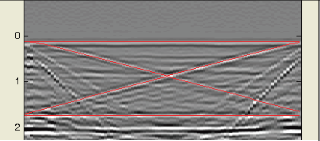
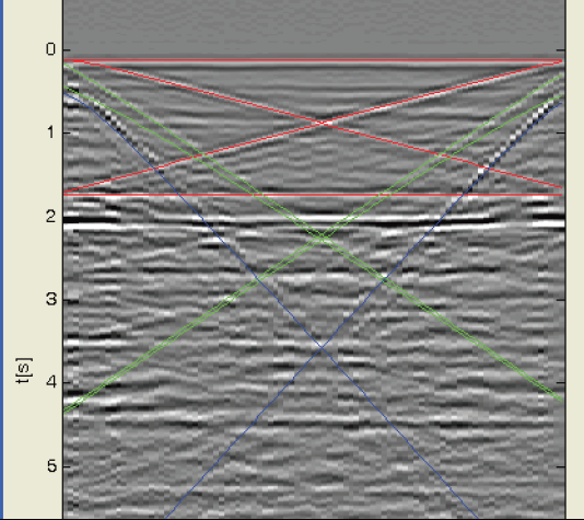
Selection and display of events

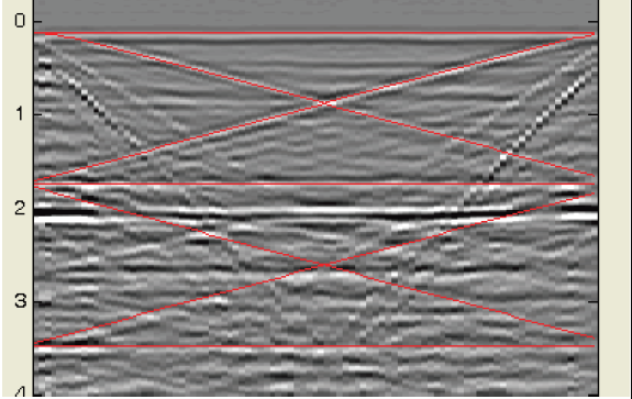
After entering speeds and “activating” the respective speed, the calculated reflection times are displayed in the left image as colored curves. Example: vpx with 5700, activated, in view 1, with display in left image (displ refl x)

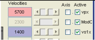
Example: vpx, mode converted wave and vs1x switched on

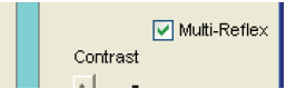
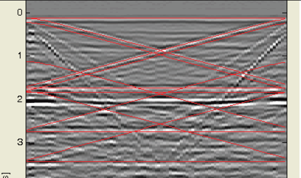
Example: vpx and multiple reflection switched on. Note: Multiple reflection can only be activated for the p-wave.

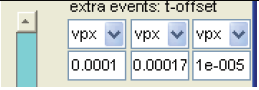
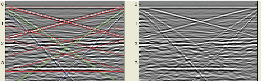
Example: vpx without multiple reflection but with 3 extra events that form with vpx and have a different initial delay.

Representation of the calculation

After changes in the parameters or when selecting the B-scans or views, the results are immediately calculated and displayed in the right B-scan. For this you can select which reflection should be suppressed. Example: xt-Slice 33 from the example data set

Execution of the calculation for all B-images and all views

The velocities in the menu can be set separately for each slice. By pressing the “Reset Velocities” button the velocity used for the first slice of the currently selected view can be transferred to the other slices of this view.

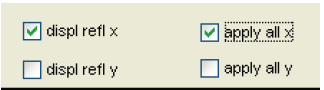
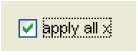
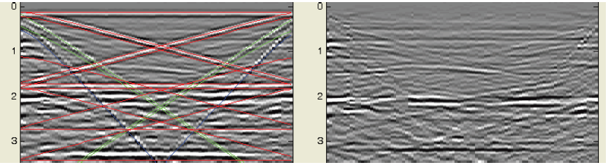
The selection of the wave direction to be suppressed can be specified separately for each view. It turned out that sometimes it makes sense to calculate all B images of view 1 with “apply all x” and all B images in view 2 with “apply all y”.

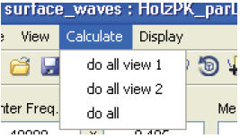
The calculation of all B-images is simply done via “Calculate” -> “do all view 1” and so on. You can follow the continuous result status in the lower right corner of the main menu.

The results are not displayed but have to be saved.

Save data

The calculated results are saved by “File” -> “Save Result Data” in ghk format and can be used immediately in other programs or be visualized by “Display” -> “Browse Results” by Browser.

Save project settings

The changes in the menu settings and the set velocities and modes can be saved as “File” “Save Settings” and read in again later.

Supplements:

The selection of a view (View1 or View2) automatically selects the velocities in the upper right main menu, since the changes in the curve are immediately recognizable by the reflections at the right and left ends of the respective coordinate axis. The changes to the propagation across the set view can only be recognized as a parallel shift of individual lines. As a short hint: the velocity in the transverse direction of all transverse B-images can be adjusted proportionally on the sliders. If you want to change the velocity in a single cross slice, press the button “single edit”. The position of the cross plane is shown in the picture and can then be adjusted with the 2nd slider. The adjustable velocities are then dark colored.

supplements

Analysis of wave detection with anisotropy