Phase Detection on Predefined Geometries

Description with an example

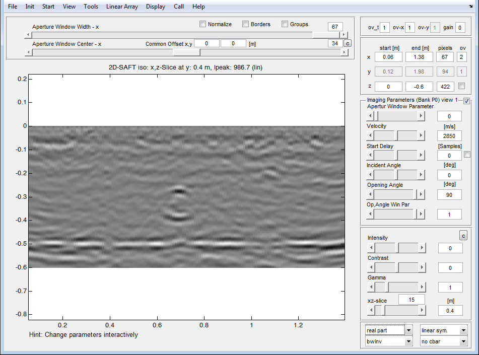
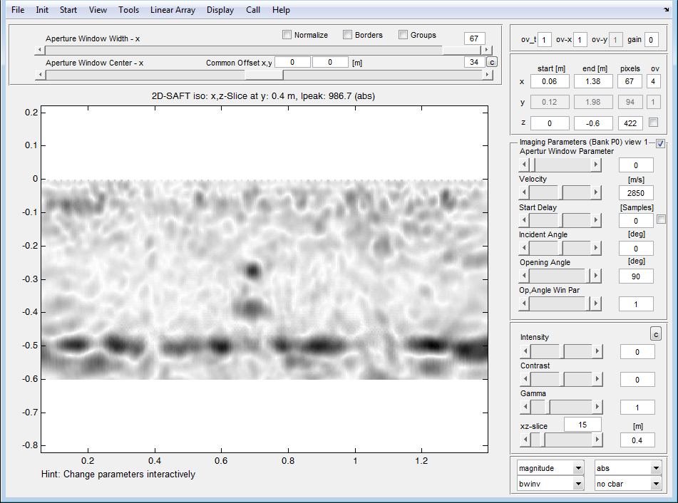
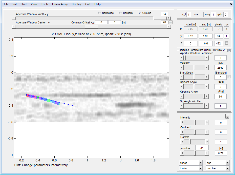
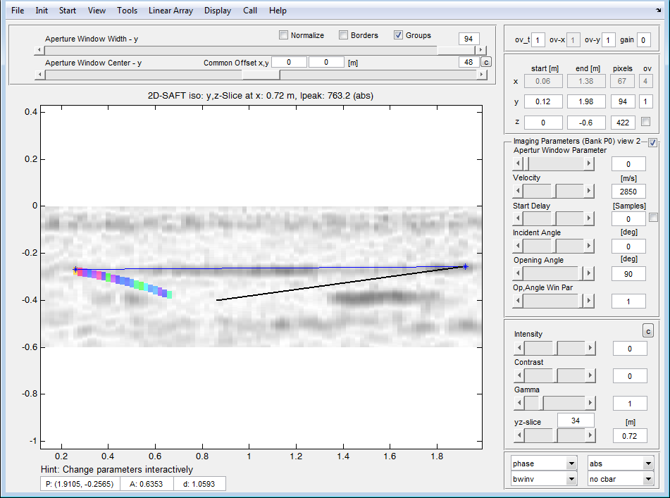
Below, the principle of phase evaluation is carried out at predetermined geometry information on a sample data set. It should be noted that the pictures are examples whose physical background is not evaluated here, and the results do not represent actual remuneration, since the choice of parameters and the phase values are arbitrary. First, the data is loaded and reconstructed by the known scheme. The interactive reconstruction of a scan line then looks for. Example like in picture 1 and 2. Filtering is set to 10-100kHz with the filter parameter 0.5. Figure 1: Real part of the 2D reconstruction, image 2: Sum.

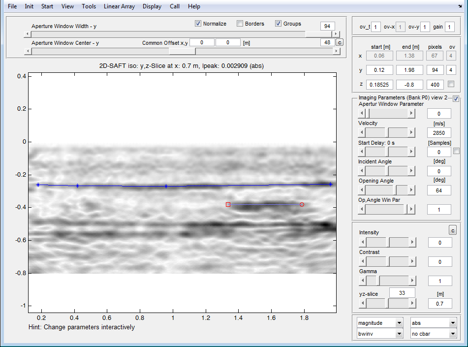
Using the geometry editor now the top edge of a cladding tube is generated. Called by: Tools -> Geometry Editor.

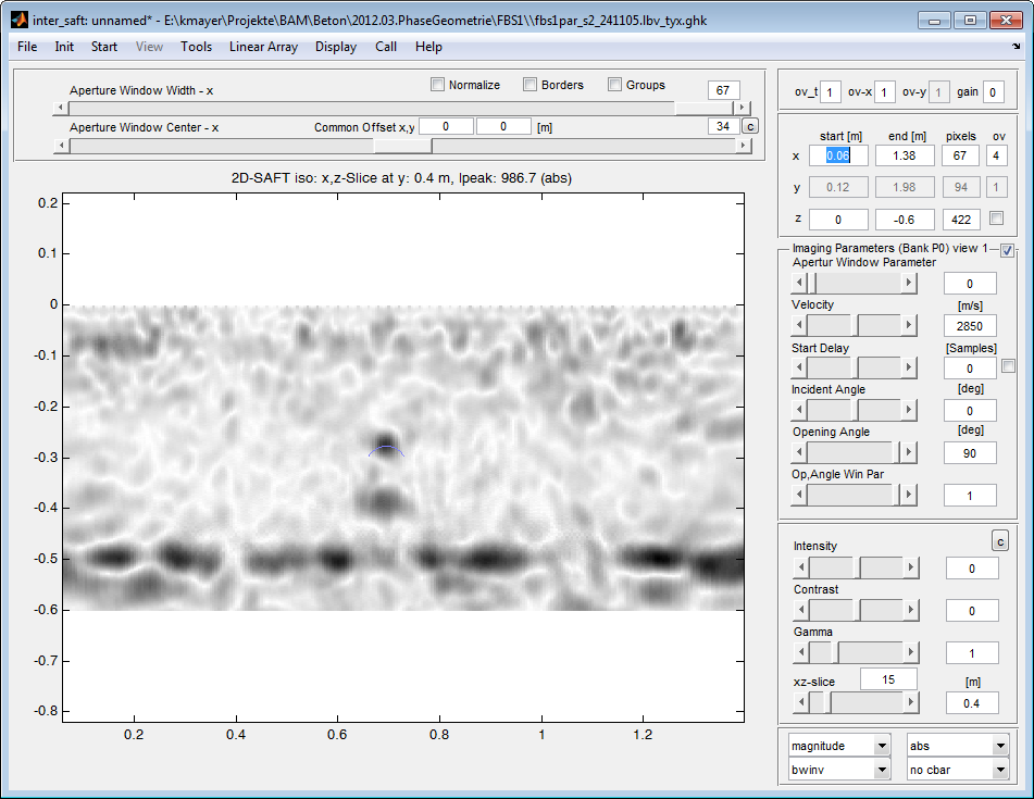
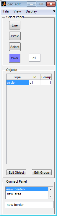
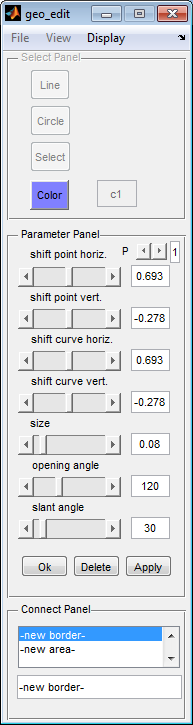
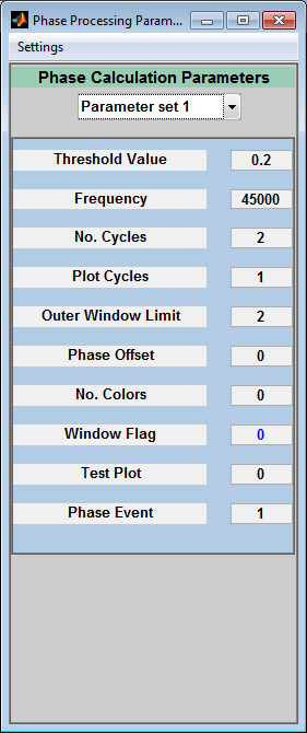
Parameters of the circle: Type: Circle, Group 1, opening angle 120° , slant angle 30° , size 0.08 The circuit is triggered by clicking on Circle and then by the definition of the upper vertex (click left mouse button) and the definition of the lower vertex (right click: defines the point and ends the input mode) generated. The parameters are then adjusted by the button ‘edit Object’ manually. It is important that the object of a group (here 1) is assigned. By File -> Exit in the geometry editor Geometry is to inter_saft finally handed over and the editor is closed. (Note: while the geometry editor is open, the view (View) can be set only in the geometry editor.) The geometry is now placed firmly in place and in all slices. It is displayed in inter_saft until Display -> Display Groups is on. The phase is calculated on this geometry, when the bottom right of the main window is placed at realpart or magnitude the selection of phase.

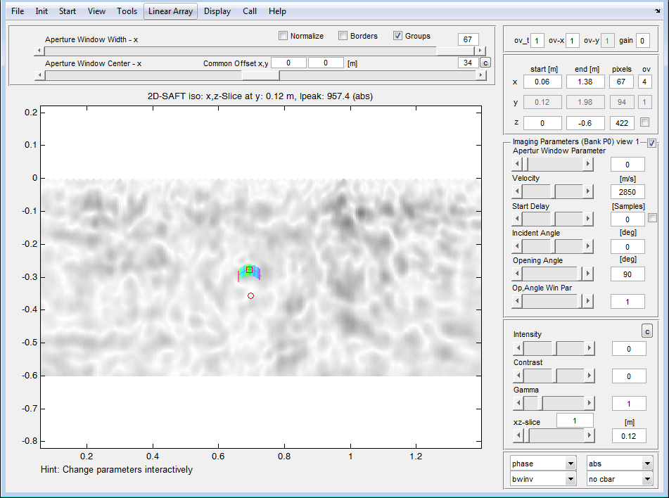
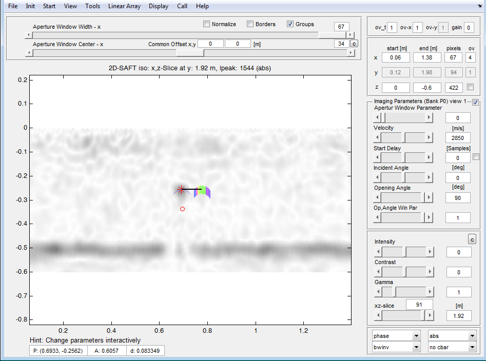
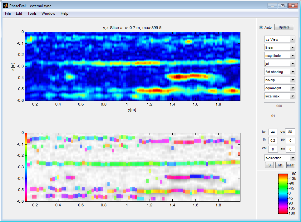
Since one can not assume that the tube (as in this example) are always in the same place in all disks, you can move the position of the generated geometry for each slice. For this purpose, the following scheme is used. One chooses in the XZ view (View xz), the first disk, in which the cladding tube can be seen, and pushes the position of the geometry with the mouse so that the top edge is positioned correctly (in this example: disc 8). Then you choose this location as a reference point: click the right mouse button on the rectangular geometry point and displays a context -Menu:

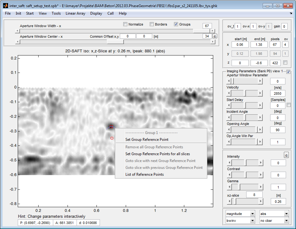
Set by Group Reference Menu the point is fixed in this slice, and characterized by a red star

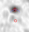
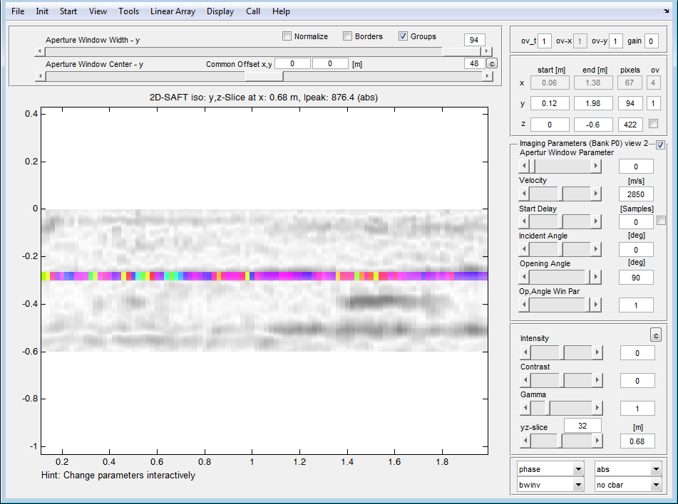
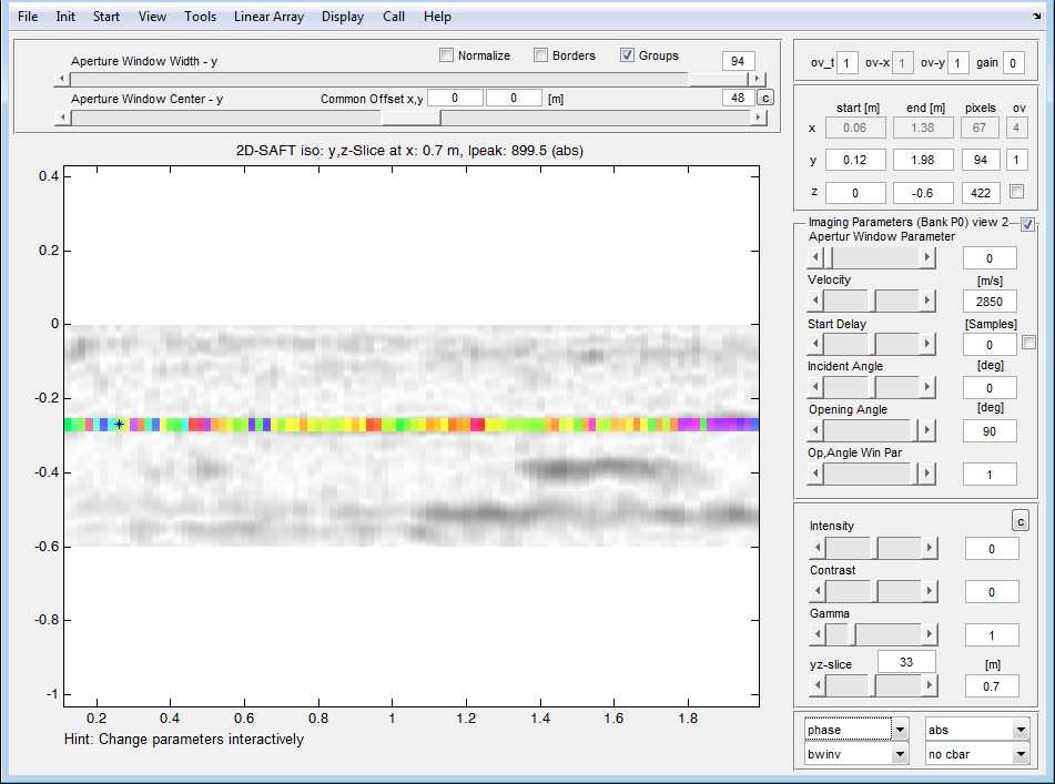
In the other view (View yz), the reference point is marked by a blue star.

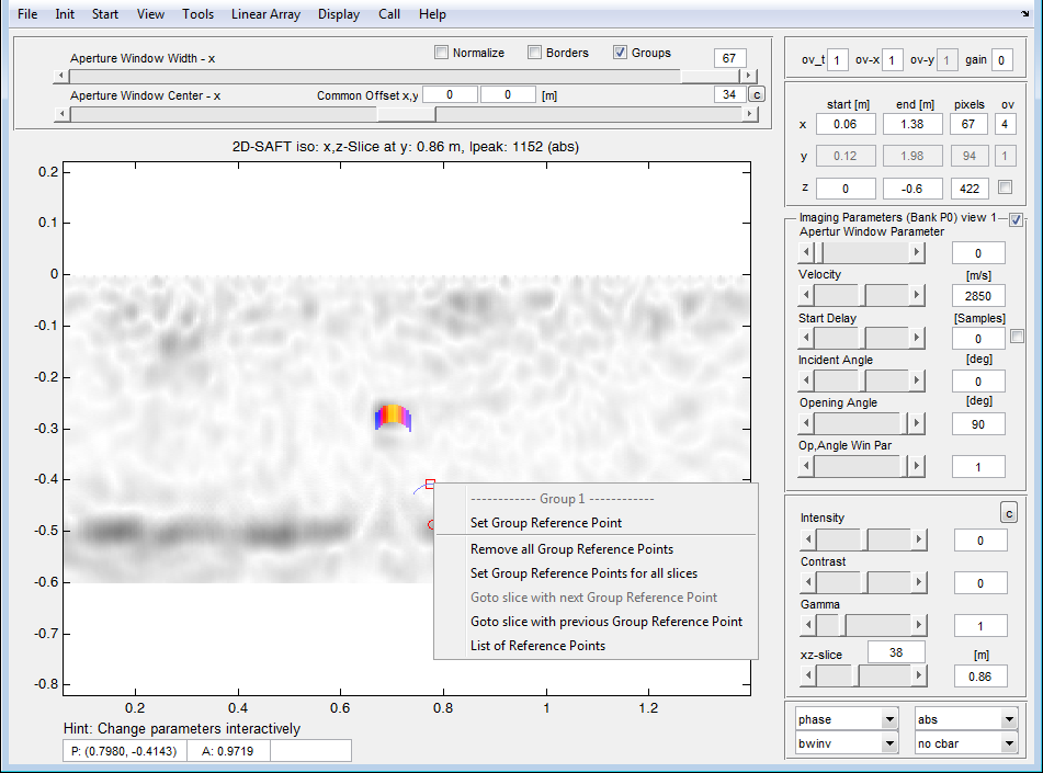
You can now move the curve in another xz slices and put more reference points. For example, in slice 38, the reference point was set arbitrarily and deliberately wrong. This has the consequence that in the yz view, a reference curve is formed which is inclined in space (and thus obliquely in the YZ view). The xz slices 8-38 are pushed to the predetermined by the reference curve points. The phase is calculated only between the 1st and last reference point.

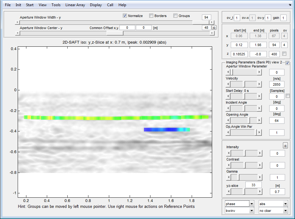
In the yz view you can now push manually the reference point of the slice 38 with the mouse in a better position with the x-position in this list can not be pushed. Again, you have in the xz view the disc with the reference point Select (right-click, context menu -> Goto Slice with next Group Reference Point). There, the object can then be pushed in the right position. If all geometries sit in the right place, you can see the ‘Display Groups’ disengaged under display again and the phase image will appear as usual, but with the geometry as specified analysis points.

The conventional phase representation can by Call -> Sync phase evaluation are switched added. Changes to Phase parameters such as center frequency, phase offset and color table are being still in phase program, but are simultaneously returned to inter_saft and applied to the representation in inter_saft by reissue of a disc.

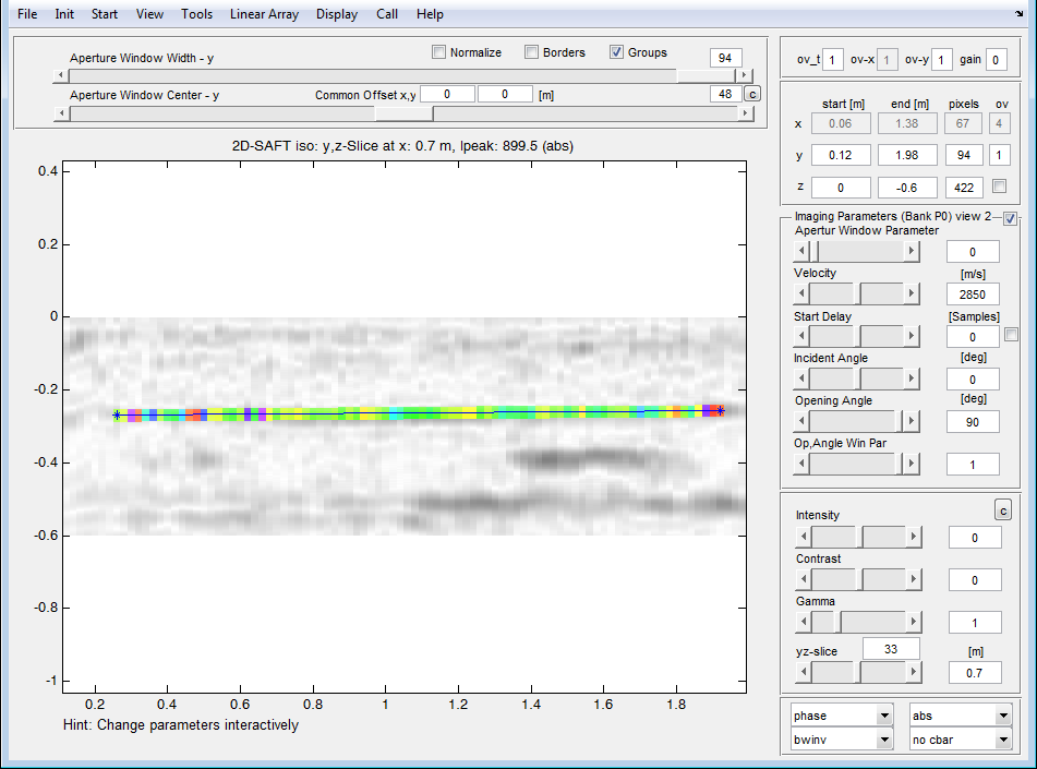
By adding other geometries the presentation can be expanded. It must be ensured that the reference lines are each assigned to a group, it is therefore necessary that objects that were created in different views (view XZ, YZ view), must also belong to different groups. For clarity, it is useful, but not necessary that the reference lines are produced in only one view. Objects of any groups belong (group 0) are not used for phase evaluation. In the pictures below, the geometry of an adjusted with 4 reference points Hüllrohroberkante and the associated phase evaluation are shown. The difference to the adaptive phase determination in Phase_eval is low.

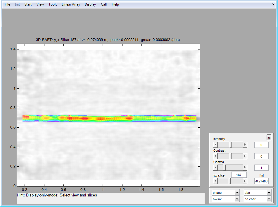
After the 3D reconstruction, the phase evaluation in the display-only mode can be used. The geometries are shown here in the C-image.