Imaging of Wood Data With the Wood Geometry Design Editor
Preparing the material properties
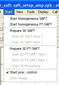
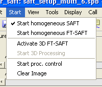
To work with the Wood Geometry Design Editor the more complex handling of the process control list is necessary. To bring InterSAFT into that mode you have to mark “Start -> Start proc. control”
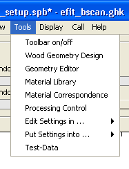
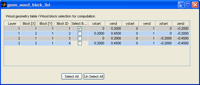
In order to do calculations with data from Wood Geometry Design Editor select “Tools ->Wood Geometry Design” to open the editor window and define the material properties of any of the blocks in each layer.
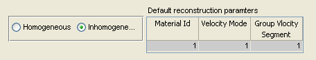
There is the possibility to start with a homogeneous material setting in the top of the window.
The material properties are given by using materials from the material library which are extracted in the material Correspondence list.
The index of the material in the correspondence list is used to connect blocks with materials. Within the correspondence list a material can appear at different places with different crystal orientation angels. So, if a user needs the material with different orientation angles, user has to assign material indices to the same material but with different crystal rotation angle parameters.
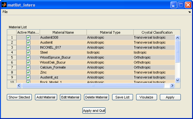
Material library
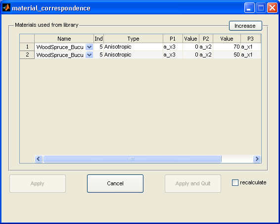
Material correspondence list
For anisotropic imaging some more parameters have to be supplied such as wave type (velocity/mode) and group velocity segment. These two parameters description is as follows. Definition wave type (Velocity/Mode) parameter which has to be used for imaging: The imaging algorithm which is used can handle only scalar waves. Therefore it is necessary to select the wave type. In some anisotropic material you have to differ between qP (Pressure) and qS1 (quasi shear 1) and qS2 (quasi shear 2). Because of the difficult structure of some of these waves one has to select parts of the group wave velocity diagram for imaging. These parameters have to be defined in the wood geometry design editor for any block:
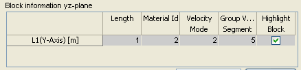
Definition Velocity/Mode and Group Velocity Segment Parameters:
Velocity/Mode |
Group Velocity Segment |
|---|---|
qp - wave |
Minimum of group velocity |
qs1 |
Maximum of group velocity |
qs2 |
Select a segment of the Group Velocity diagram |
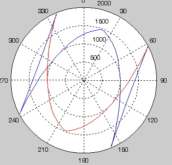
Example: Material: wood spruce
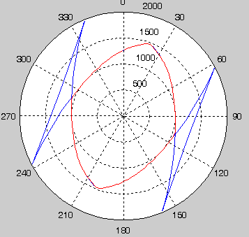
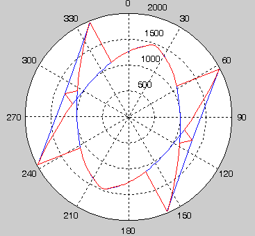
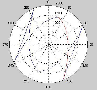
(Left) : Parameters 2, 1 Minimum of qS1; (Middle) : 2,2; Maximum of qS1; (End): 2,3
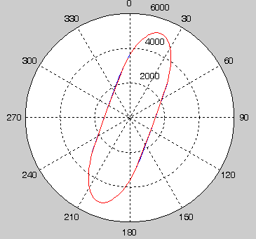
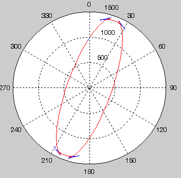
(Left) : 2,5 ; (Middle) : Parameter 1,0 P-Wave; (End) : 3, 1 Minimum of qS2
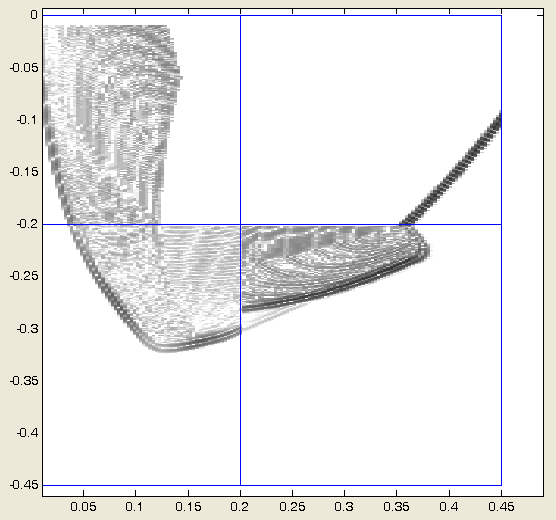
During calculation a plot window shows the selected part of velocity diagram. (Work in progress).
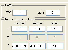
Preparing the reconstruction area
To get an overview to the data it is useful to do some homogeneous calculations first. This should be done with the -> Start homogeneous SAFT call from the main menu.
This calculation is interactive, that means changes in the parameter settings are visible almost in real time (depending on the resolution and the computer speed). The data area and the homogeneous background velocity can be adjusted interactively so that an overview of the image is displayed.
Generating the processing control calculation
Using the apply button in the geometry design editor starts the generation of the connection lists between all blocks which are selected to be processed on the way of the waves from the measurement surface to the reconstruction areas. Remark: It is possible not to calculate all blocks, but for testing purposes you can select the blocks which are of most interest.
The process control list is generated automatically. The result can be seen in the processing control menu: Main -> Tools -> Processing Control
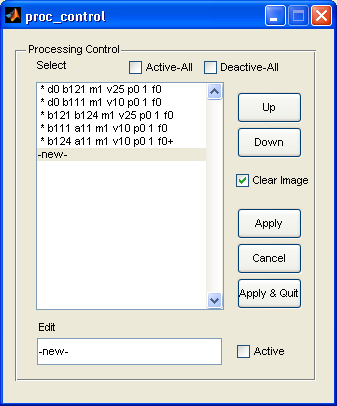
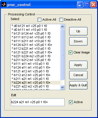
This list, which is already known from previous version, can be rather full, depending on the structure of the wooden bar. The list contains the processing steps in that order, which is necessary that data are available in the step when they are used. Calculation can be separated into groups:
Transportation of measured data to a border: d0 b121 … Transportation of border data to another border: b121 b124 … Imaging of border data to an area: b124 a11 ….
The parameters are defined as follows, explained by an example:
Selection |
Source |
Destination |
Material |
Velocity |
Parameter Bank |
Factor |
Displ. Area |
|---|---|---|---|---|---|---|---|
d0 |
b121 |
m1 |
v21 |
p0 |
1 |
f0 |
|
b121 |
b124 |
m1 |
v21 |
p0 |
1 |
f0 |
|
b121 a11 m1 v21 p0 1 f0 |
|||||||
This means: from the list of all steps, the marked as active lines are processed. Lines which are not marked are ignored. In the first step, the measured data have to be assigned to a border. (Here d0 -> b121). If the border is part of the measured aperture, the data are copied to the data part of the border. Material parameters and velocities are ignored. If the data and border are not connected, the data have to be processed by wave propagation with the given parameters to the border. The parameters are:
- Selection:
The mark “*” indicates that the processing step is activated. If a processing step is deactivated (by unselecting the flag “Activate”), the data of that process are not generated, and all the depending processing steps are skipped.
- Material:
Index of the material into the material correspondence list. If material index = 0, the isotropic material described by the main menu is used
- Velocity:
v0: Velocity of the main menu is used
vNNNN: (if NNNN is a number greater 10) it is uses as isotropic velocity for the processing (e.g. v5900 for steel)
vXX: XX gives the group velocity selection (p,s,qs) and the part of the group velocity as defined in the previous section
- Parameter Bank:
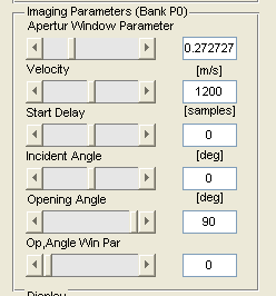
For some type of calculations it is possible to use different settings for the main menu parameters (Orientation angle, window functions a.s.o.). Within the main menu (Tools -> Edit Settings in. , or Tools -> Put Settings into .) the parameters can be stored into banks (bank0 . bank4). The Setting stored in bank n can be assigned to a processing step by adding the bank to the p-parameter. Parameters from Parameter Bank are only used by calculations from data to the total reconstruction area. This means the source must be “d0” and the destination must be “a0”.
- Factor:
This number is multiplied to the result of a reconstruction process in order to ajust different areas to each other.
- Display Area:
Usually user want to view the result of a reconstruction within the main window, therefore the default value is f0 (stands for figure 0). But it is possible to put the intermediate result of one calculation step into a separated figure. The identification number of a figure must be specified correctly, because the last image assigned to a figure overwrites the previous one. The images into the main window are accumulated usually. This is achieved by a “+” at the end of a figure number (e.g. f0+). The process list is generated automatically in this way. If you omit or delete this “+”, the image produced in that processing step deletes all images in the area of previous calculations.
- Number scheme of borders and areas:
Processing lists obtained from the wood geometry design window have a unique numbering. All border numbers have 3 digits.
bijk :
i: the layer of the block counted from the measured aperture
j: id of the block in the layer i (from left to right 1…9)
k: border id around the area: 1: top, 2:right, 3: bottom (not used), 4:left
All area numbers have 2 digits:
aij : having the same meaning as for blocks
Example: Assume xz-plane is the simulation or reconstruction plane, then the borders and areas are defined as shown in the following figure. Area is denoted with - a(layer, block in x direction), border is denoted with b(layer, block in x direction, edge number of the block in clockwise direction starting with top edge)
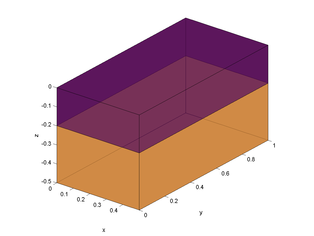
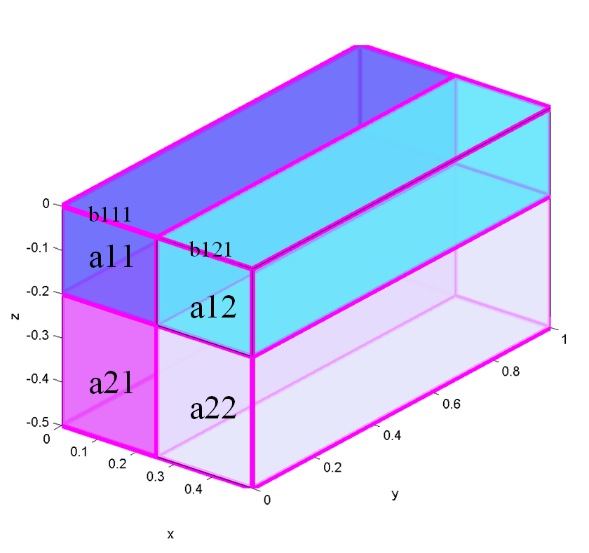
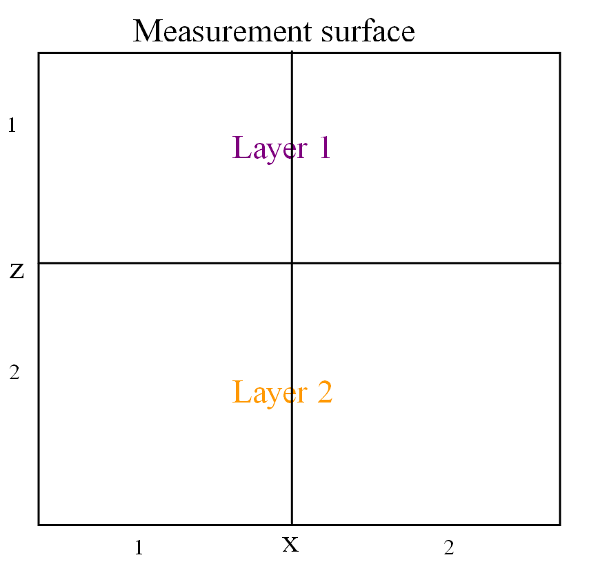
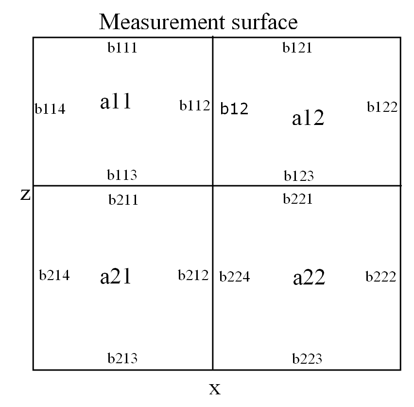
(3): xz-plane layers: 2D representation; (4): xz-plane areas and boundaries: 2D representation
Starting the Processing control calculation
To start the processing calculation for the first time, “Menu-> Start Processing Control”? has to be activated. If this flag is set, the processing is repeated automatically if a parameter has changed within the processing flow control and if the respective “apply”? button has been pushed. The result is displayed in the main window and ” if selected ” all figures on the way to the result are updated. If the number of a figure of a previous calculation is dropped from the list, the figure must be closed manually; it is not updated by any information.
Using the test mode
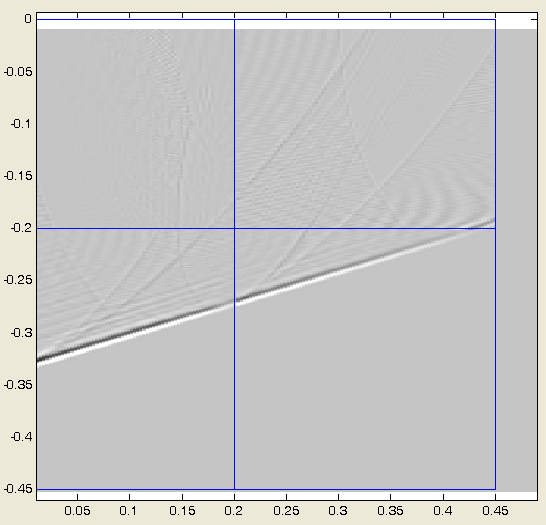
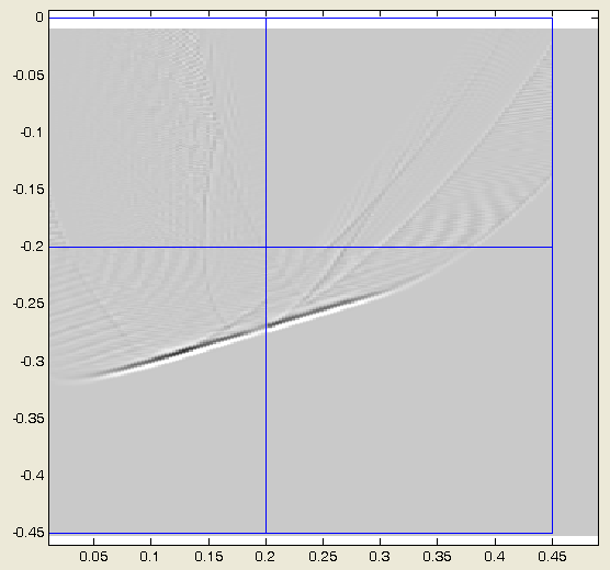
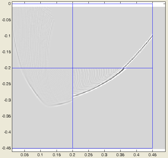
From the main menu “Tools -> test-data”? a synthetic data arrangement can be switched on. The data replaces the measured data completely, having the same measurement parameters like the original data. This data can be used to test the algorithm and to see effects of interactive parameter settings. The “Tools->Options” menu can be used to control the parameters of the test data. The example is given for a receiving plane wave under the angle of 30° with an RC2 impulse at a frequency of 80 kHz.
Example:
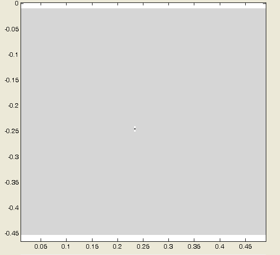
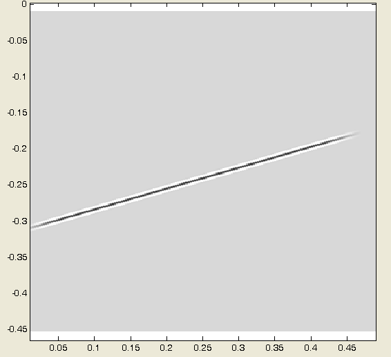
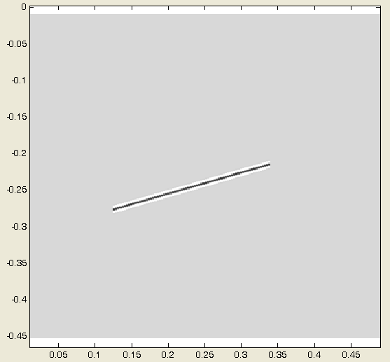
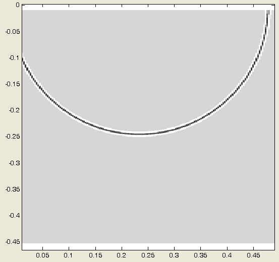
(L): Test data, (SAFT with beam opening angle = 0° ), aperture width = 0; (M): Test data, aperture width 100° , with aperture window function; (E): Test data, aperture width 50%, without aperture window function
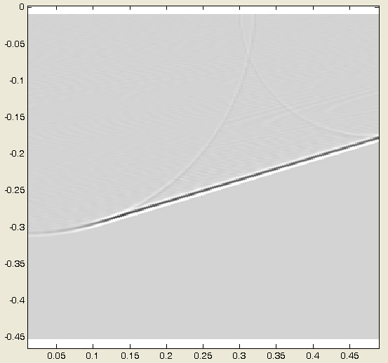
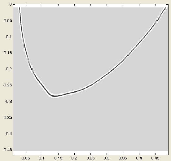
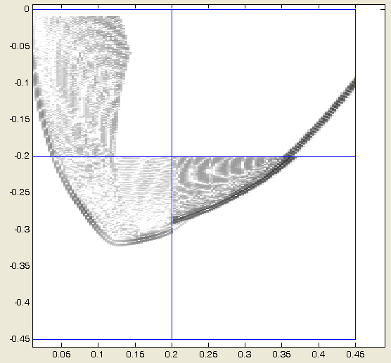
SAFT-Reconstruction of test data above, homogeneous isotropic background medium for SAFT imaging
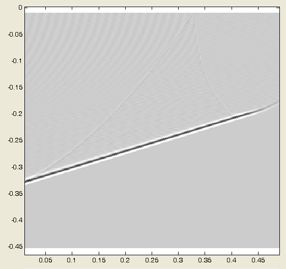
SAFT-Reconstruction of test data above, homogeneous anisotropic background medium for SAFT imaging
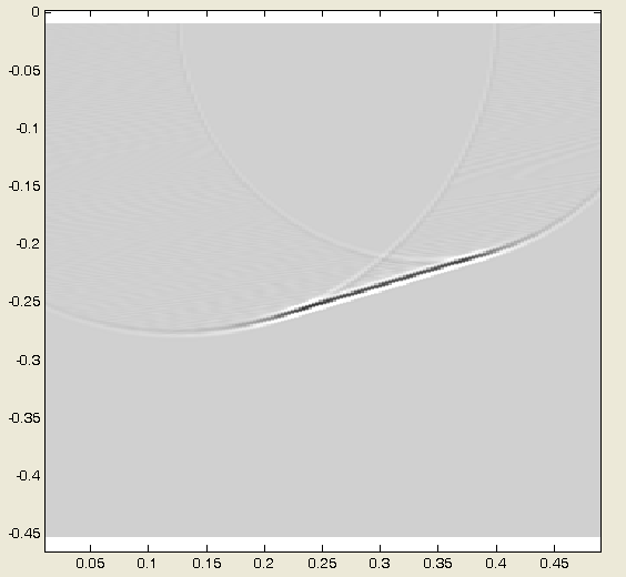
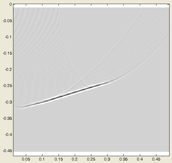
SAFT-Reconstruction of test data above, homogeneous anisotropic background medium for SAFT imaging, using processing control and border to border propagation
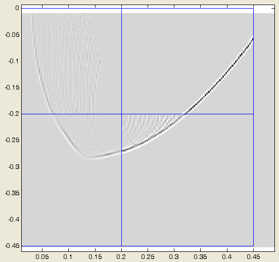
(Center):SAFT-Reconstruction of test data above inhomogeneous anisotropic, block 2,2 has changed material orientation. Original 70° , now 50° . Left: linear range, middle log 60 range.; (End): Block 2,2 now has 30° orientation. “Anisotropic SAFT keeps the boundary condition”
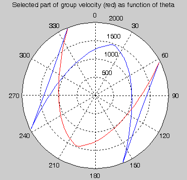
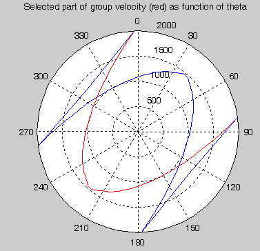
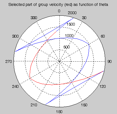
(L): Anisotropic group velocity of Wood Spruce: orientation of 0° ; (M) : Orientation 50° ; (E): Orientation 30°